Useful New Functions in Recent Microsoft Excel Updates

Microsoft is transitioning its Office program from a one-time purchase price to a paid monthly rate. One of the advantages of the new payment structure is the ability to always have access to the latest Microsoft Office update, without ever having to pay for an upgrade. If you’ve been wondering about the value in this, you may be interested to hear about a recent Microsoft Excel update. With version: 16.0.6568.2025, released in February 2016, Excel now includes six new functions. I know I’ll definitely be using some of these in the future! Here’s a quick breakdown of the new functions the Microsoft Excel update.

Note: This post may contain affiliate links.

If you’re on the monthly plan you should already have access to these functions. If you’re not on the monthly plan and interested in learning more, check out Microsoft’s Office options here.

New Functions in Recent Microsoft Excel Updates

1st New Function in Microsoft Excel: CONCAT

In a previous post we showed you how to combine cells in Microsoft Excel. The new CONCAT function will also combine (or concatenate) cells.

CONCAT Formula Syntax

=CONCAT(item1, item2,…)
To use the CONCAT formula you type =CONCAT and then, in parentheses, add the items you want to join together. The items you add can be cells, text or a mix and should be separated by commas.

CONCAT Examples

• If you want to combine cells A2 and B2 you would use the formula:
  =CONCAT(A2,B2)
• To combine cells A2 and B2 and place a comma in between them you would write:
  =CONCAT(A2,”, “,B2)
  Note that the characters you’re including, a comma and space, are enclosed in quotation marks. You don’t use quotation marks when referencing cells.
• To combine text and the value in a cell you could write:
  =CONCAT(“The result is “,A2)

CONCAT Formula Notes

• This formula replaces the older CONCATENATE formula which still appears in older versions of Excel.
• You can include up to 253 arguments in this formula. In other words, you can join up to 253 items.
• If the resulting field is more than 32,767 characters it will return an error.

2nd New Function in Microsoft Excel: TEXTJOIN

The TEXTJOIN function is similar to the new CONCAT function but it adds a delimiter (a character you specify) in between the items you’re joining. If you want to join several words but want a space in between each one the space would be your delimiter. Some other common delimiters are a comma (,), a comma with a space after it (, ) and an ampersand (&). In addition to having to specify what you’d like to use as a delimiter you also have to tell Excel how you want it to handle empty cells. Do you want to add the delimiter and an empty space or skip over it completely? Let’s look at a few examples.

TEXTJOIN Formula Syntax

=TEXTJOIN(delimiter, ignore_empty, item1, item2,…)
So, to use this formula you type =TEXTJOIN and then, in parentheses first write the delimiter you’d like to use (enclose this in quotation marks), then, after a comma, write TRUE or FALSE (NOT in quotation marks) and then add the items you’d like to join, separated by commas.

TEXTJOIN Formula Examples

• To join cells A1 and B1, skipping over and empty cells, with a space in between you’d use:
  =TEXTJOIN(“ “,TRUE,A1,B1)
• To join cells A1, B1, C1 and D1 using an ampersand (&) and leaving an empty spot for any blank cells you’d type:
  =TEXTJOIN(“&”, FALSE,A1,B1,C1,D1)
  Let’s say cell A1=A, B1=B, C1 was empty and D1=D. The formula above would return: A1&B1&&D1 . Notice since we used FALSE for the ignore_empty argument a delimiter was still used before and after C1 even though it was an empty cell.

TEXTJOIN Formula Notes

• You can include up to 253 arguments in this formula. In other words, you can join up to 253 items.
• If the resulting field is more than 32,767 characters it will return an error.

3rd New Function in Microsoft Excel: IFS

If you’ve ever used a nested if statement as shown here on the MBA Excel blog, you’ll be happy to learn about this new formula in the Microsoft Excel update called IFS. IFS is way to create an if/then function with multiple if statements.

IFS Formula Syntax

=IFS(if1,then1,if2,then2,…)
To create several if/then statements type =IFS then, in parentheses, add the if part of the statement, followed by the then part of the statement, separated by commas. Repeat this for each if/then statement you want to use, separating each new set from the previous with a comma.

IFS Formula Example

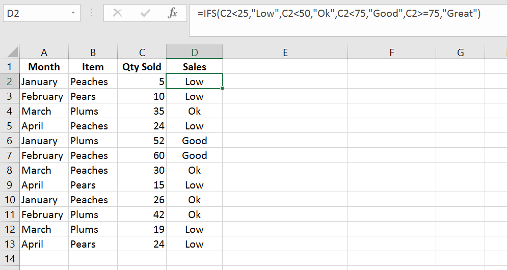
In the following image the IFS function is used to categorize sales by “Low”, “Ok”, “Good” and “Great” based on the number of pieces of fruit sold. The function used is:
=IFS(C2<25,”Low”,C2<50,”Ok”,C2<75,”Good”,C2>=75,”Great”)
This formula will return “Low” for any value below 25, “Ok” for values of 25 through 49, “Good” for values 50 through 74 and “Great” for anything 75 or more. In the example we’ve copied the formula down column D so you can see the results as it evaluates the values in column C.

IFS Formula Notes

• To create an “else” statement, specify a positive result for the final if statement such as 1=1 or writing TRUE.
• If none of the conditions return a true value, you will get an error message.
• You can list out up to 127 pairs of if/then statements in the IFS function.

4th New Function in Microsoft Excel: SWITCH

The new SWITCH function in Excel allows you to compare an expression against several values and return a result corresponding to the matching value. This may sound a bit confusing but should be clearer in the example below.

SWITCH Formula Syntax

=SWITCH(evaluate_range,criteria1,result1,criteria2,result2,…)
To use the SWITCH function you write =SWITCH and then, in parentheses, write the expression you are evaluating followed by the value and result to return if the expression matches this value, separated by commas. You can then add additional values/results separated by commas. After you’ve entered all your value/results combinations you can also add a default result if none of the values match. (The default result is optional.)

SWITCH Formula Examples

In the example below we use the SWITCH formula to change the month name to a number (note there are other ways of doing this using the LINK format function). The function used is:
=SWITCH(A2,”January”,1,”February”,2,”March”,3,”April”,4,”May”,5,”June”,6,”July”,7,”August”,8,”September”,9,”October”,10,”November”,11,”December”,12,”???”)
Note that the month word is text so is placed in quotation marks but the result we want returned is a number so we don’t need to enclose the results in quotation marks. Also note that we want the cell to display ??? when no match could be found. This allows us to quickly check for errors in a large document.

5th New Function in Microsoft Excel: MAXIFS

If you’ve used the MAXIF function before you’ve probably ran into an occasion where you wanted to reference more than one criteria. You used to have to create a formula like the one found on the contextures blog to achieve your result. Now the MAXIFS function allows you to use several if criteria. The example below shows you how to use the MAXIFS formula.

MAXIFS Formula Syntax

=MAXIFS(minimum_range,criteria1range,criteria1,criteria2range,criteria2,….)
To use the MAXIFS function in the recent Microsoft Excel update you write =MAXIFS and then, in parentheses, you first enter the range you want to evaluate for the maximum value. Then, after a comma, you enter the range you want to evaluate for your criteria, another comma and the expression to evaluate for the range. If you have more criteria you can enter them after the first, separating them all by commas.

MAXIFS Formula Examples

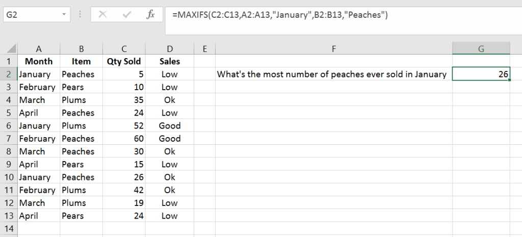
In our spreadsheet example we use the MAXIFS function to evaluate the maximum number of peaches that were ever sold in January. The expression we use is:
=MAXIFS(C2:C13,A2:A13,”January”,B2:B13,”Peaches”)
Note that the first thing entered in the parentheses is the range C2 through C13. This is the range that contains the maximum number we want to find. Next we enter the first range we want evaluated, A2:A13 and the criteria for that range, “January”. (Note that January is enclosed in quotation marks because it is text.) Then, after another comma, we enter the next range, B2 through B13 and the criteria to evaluate against, “Peaches”.

If more data was going to be entered in the spreadsheet it may make sense to evaluate the data in the all the rows. To do this we would change the formula to read:
=MAXIFS(C:C,A:A,”January”,B:B,”Peaches”)
Notice that instead of specifying the range C2 to C13 we wrote C:C. This tells Excel to evaluate the entire column. Since we’re evaluating the entire column for the maximum value we also must evaluate the entire column for each criterion.

MAXIFS Formula Notes

• If the ranges specified don’t match in size and shape the MAXIFS function will return an error value.

6th New Function in Microsoft Excel: MINIFS

Similar to the MAXIFS function the MINIFS function can evaluate a range for a minimum value when corresponding ranges meet specified criteria.

MINIFS Formula Syntax

=MINIFS(minimum_range,criteria1range,criteria1,criteria2range,criteria2,….)
To use the MINIFS in the recent Microsoft Excel update write =MINIFS and then, in parentheses, enter the range you want to evaluate for the minimum value. Then, after a comma, enter the range you want to evaluate for your criteria, another comma and the expression to evaluate for the range. If you have more criteria you can enter them after the first, separating them all by commas.

MINIFS Formula Examples

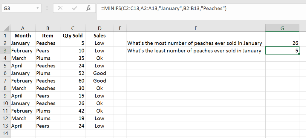
Using the same example as above we can evaluate the minimum number of peaches sold in January with the formula:
=MINIFS(C2:C13,A2:A13,”January”,B2:B13,”Peaches”)
The formula is the same as above except the function MINIFS is referenced at the beginning.

MINIFS Formula Notes

• Just like with MAXIFS, if the ranges of cells specified don’t match in shape and size the formula will return an error.

Conclusion

With quite a frugal personality I had a hard time accepting the idea of paying monthly for Microsoft Office. The benefit of always having the latest upgrade didn’t seem significant to me. After all, I can get on a computer running Office 2007 and still work fine. However, now that I have seen some the recent upgrades and these new functions in the Microsoft Excel update I’m glad to be on the Microsoft Office 365 plan. I know I’ll be using some of the functions above pretty regularly. If you have the latest Office check these out. If you have any difficulty using them leave a comment below so we can help out!

References

• CONCAT Function – Microsoft Website
• TEXTJOIN Function – Microsoft Website
• IFS Function – Microsoft Website
• SWITCH Function – Microsoft Website
• MAXIFS Function – Microsoft Website
• MINIFS Function – Microsoft Website