How to Use Excel Text to Columns To Separate First and Last Names

Have you ever had an excel spreadsheet in which you’d like to split one column into two or more? For instance, say you have a column with names and you want to separate the first and last names into two separate columns. Excel has a built in function called text to columns which enables you to do this very quickly. In this post we’ll show you how to use excel’s text to columns function to separate names.

Separate First and Last Name Using Text to Columns

Open the spreadsheet that has a column of first and last names. Now, assuming this column is first and last names only with a space in between, follow the steps below to separate the first and last names into separate columns.

When you use text to columns your first and last name column will become 2 columns. If you have columns to the right of your name column you’ll have to insert a blank column so you don’t lose any information. This blank column will become your last name column.

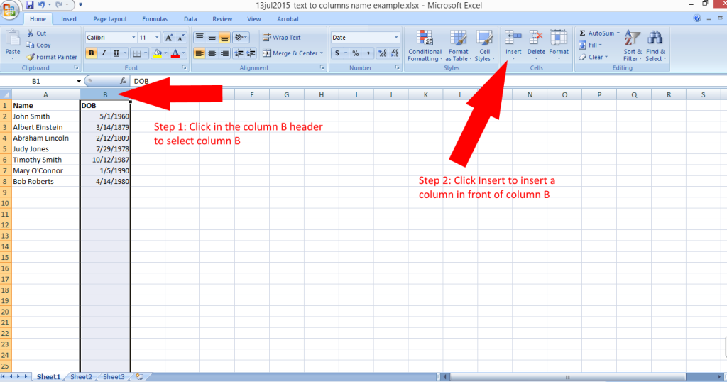
To insert a blank column select the column to the RIGHT of where you want to put the blank column by clicking in the header row. In our example, we want to put the blank column in between columns A and B so we select column B by clicking in the header area of column B. Then click insert from the menu and a new column will be inserted.

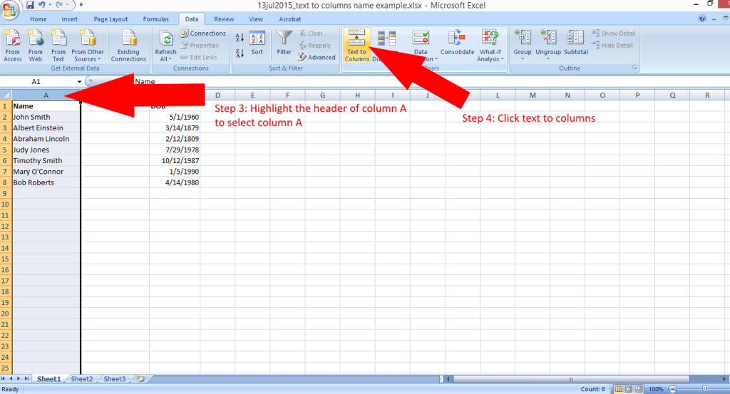
Next, select the column with the first and last names that you want to separate. In our example, that data is in column A so we select column A by clicking in the header area around where it says A. Then, go to the data menu and click text to columns.

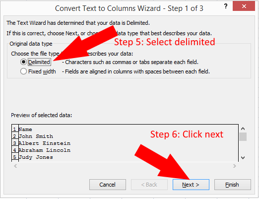
This will open the wizard that walks you through the text to column function. There will be three screens to go through. In the first, you’re going to tell excel how your information is separated. Since our first and last names are separated by a space, we’re going to select delimited, which means that we want the text to be separated at a specific character. In our example, the character being used as a separator is the space. Click next.

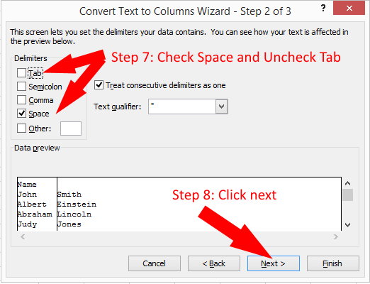
Since we are separating our data at the space we check space and make sure the other characters are not checked. You’ll see a preview of your data in the bottom of the window so you can be sure that you’ve got the right combination. When it looks correct, click next.

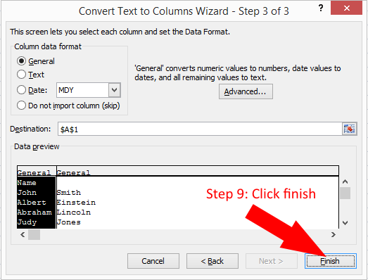
On the last screen you can identify the data types for columns. We don’t need to do that so we just click finish.

Our names are now split into two columns!

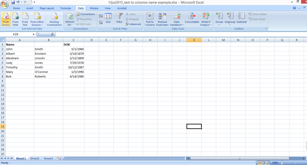
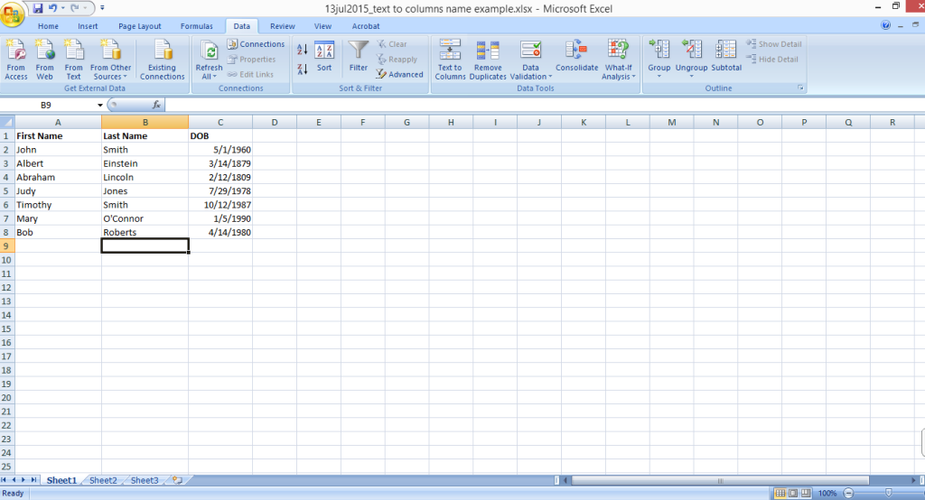
We can add a name to our column and our spreadsheet looks like this:

 

If your data is stored differently or you run into any problem, leave a comment below and we can help!

Also, check out our post on an advanced use of the text to column function where we use it to separate addresses into street, city, state and zip. And subscribe below to get alerted of new Excel and easy tech tutorials: