How to Calculate a Percent in Excel

In this article we’ll walk you show you the 3 easy steps to calculate a percent in Excel or a calculate a percent change in Excel. First, we’ll review the basics of what is a percent and what is the formula to calculate a percent. Then we’ll show you how to calculate a percentage in Excel. Finally, we’ll explain the formula used to calculate a percent difference and show you how to calculate a percent change in Excel. Let’s do it.

Note: This post may contain affiliate links.

What is a Percent?

According to Wikipedia:

In mathematics, a percentage is a number or ratio expressed as a fraction of 100.

So, if you have 100 jelly beans and 10 of them are red, 10 out of 100 are red, or 10% are red.

But, what if you don’t start with exactly 100? Well, you can calculate a percentage so you know how many would be red if you had exactly 100.

Let’s say you had 500 total jelly beans and 50 are red. Ten percent of our jelly beans are still red, even though we’re referring to a bigger group.

By using percentages to refer to things we can compare groups of different sizes. It “normalizes” the group size.

How Percentages Help Us Compare Items – Example

The easiest example to think of is a grading system in a school. Lets say one week there is a test of 25 questions and the student gets 5 wrong. The next week there’s a test with 100 questions and the student gets 7 wrong. The student got more questions wrong the second week so did he do worse? Well it’s hard to compare when the tests didn’t have the same number of questions. But, if we use percentages we can “normalize” the numbers and compare them to each other, as a fraction of 100. The first week the student got 80% correct while the second week they got 93% correct. So, actually, he got a higher percentage correct and, therefore, did better the second week.

How to Calculate a Percentage

Let’s break down the definition of a percentage.

Calculate a Percent Step 1 – Calculate the Ratio

Going back to our definition from Wikipedia, let’s focus on the first part:

In mathematics, a percentage is a number or ratio expressed as a fraction of 100.

A percentage is a ratio.

So, the first step in calculating a percentage is to calculate the ratio.

Let’s say we want to figure out what percentage of our monthly income goes to our mortgage payment. We first need to calculate a ratio of our mortgage payment to our total income. We do this by dividing the “portion” of our monthly income by the “total” income:

ratio = mortgage payment ÷ total monthly income

Calculate a Percent Step 2 – Change our Ratio to a Fraction of 100

Now that we have our ratio, let’s look at the second part of the definition:

In mathematics, a percentage is a number or ratio expressed as a fraction of 100.

We now have to express our ratio as a fraction of 100.

The site, Helping with Math, describes how to do this nicely. To change a ratio to its percentage:

multiply by 100 (or move the decimal point two places to the right)

So, for our example, we can change our ratio to a percentage by multiplying by 100:

mortgage payment as percent of total income = mortgage payment ÷ total monthly income x 100%

Let’s put it all together using numbers. Let’s say our monthly income is $3,000 and our mortgage payment is $1,000. We can calculate the percentage of our income that’s going to our mortgage with this formula:

mortgage payment as percent of total income = $1,000 ÷ $3,000 x 100 % 

mortgage payment as percent of total income = 33 %

How to Calculate a Percent in Excel

So now that we know what a percentage is and how to calculate it. How can we calculate a percent in Excel?

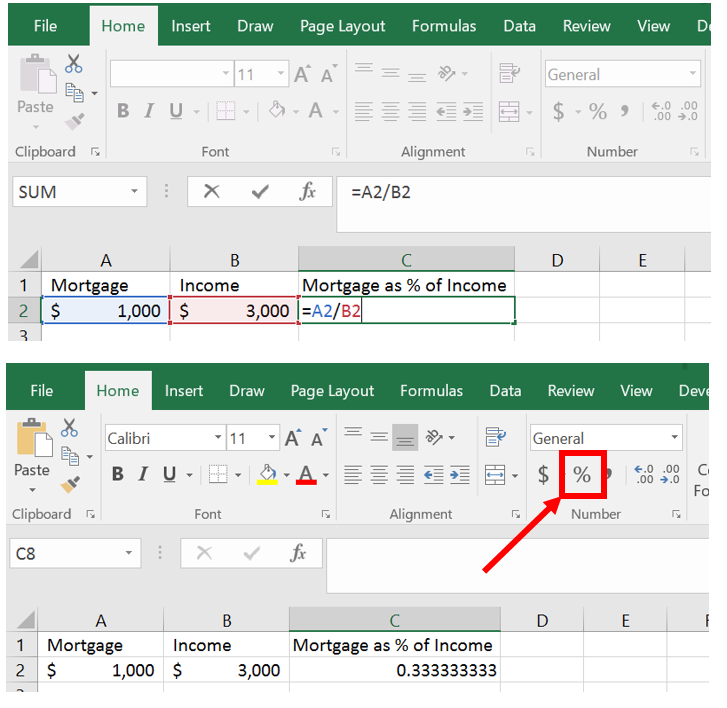
Let’s say we have an Excel spreadsheet for our home budget. In our spreadsheet we have our monthly mortgage payment and our monthly income. We want to know what percentage of our income is going toward our mortgage. We can calculate a percent in Excel like this:

In the cell where you’d like to calculate the percentage, add this formula: =A2/B2  and press enter. A2 in our case is the cell with the mortgage payment (the “portion of the whole” we want to calculate). B2 is our income in this case (“the whole”).

You’ll now see a ratio in your cell. In our case, the ratio is showing how much money we spend each month on the mortgage.

In the home menu, look for the number section and click the % button. When you click this icon, Excel calculates the percentage by multiplying the ratio by 100 and adding a % sign.

Your cell now shows the percentage of money you spend each month on your mortgage

In short, to calculate a percent in Excel:

1. type =A2/B2 (substituting the cell names as appropriate)
2. press enter
3. click the % button in the number section of the home menu

How to Calculate the Percent Change in Excel

How to Calculate the Percent Difference

Another common use of percents is to compare how much things have changed. The formula for calculating the percent change (or percent difference) between two numbers is:

percent change = (new number – original number) ÷ original number x 100%

So, if my previous income was $3,000 and I now make $3,100, what is the percent change of my income? In other words, by what percent did my income increase or how big of a raise did I get?

percent change = (new income – old income) ÷ old income x 100%

percent change = ($3,100 – $3,000) ÷ $3,000 x 100%

percent change = ($100) ÷ $3,000 x 100%

percent change = 0.033 x 100%

percent change = 3.3%

Note: One important thing to remember is that you always divide by the old number or the original number. If you use the new number by accident you’ll get a different result!

How to Calculate the Percent Difference in Excel

Now that we know what it is, let’s learn how to calculate a percent difference in Excel.

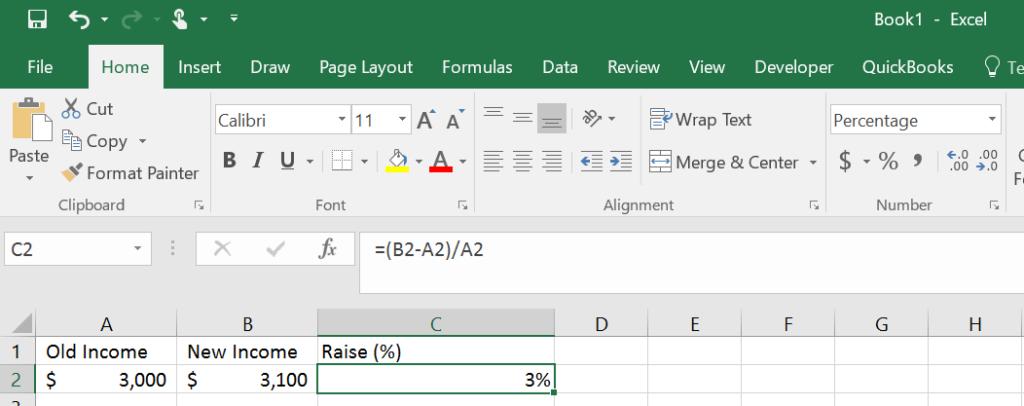
Let’s assume we’re starting with an Excel spreadsheet that has our original income and our new income in it:

Let’s calculate the percent change in cell C2. First, we need to figure out the ratio, just like above. However, the ratio is a little different. Remember, the formula for percent change is:

percent change = (new income – old income) ÷ old income x 100%

But we only want the ratio right now so we’ll remove the 100% from the end.

percent change = (new income – old income) ÷ old income

Just replace “new income” with the cell that holds your new value (B2 in this example) and replace “old income” with the cell that is holding the old income (A2 in our example).

percent change = (B2 – A2) ÷ A2

So, in cell C2 (where we want our result) we’ll type:

= (B2 – A2) / A2

Notice that we’ve typed the parentheses in the formula just as they’re shown above. This is necessary for this formula so it’s calculated in the correct order. Also note the slash is used as a division sign in Excel.

Now press enter to see the result of your formula.

Finally, let’s turn our ratio into a percent by clicking on the percent icon in the number portion of the home menu. Excel calculated the percent by multiplying by 100 and adding a % sign.

In short, to calculate a percent change in Excel:

1. Type =(B2-A2)/A2 (where A2 is the cell with the old value and B2 is the cell with the new value)
2. Press enter
3. Press the % icon in the number section of the home menu

Conclusion

By using formulas to calculate percentages and percent changes in Excel you can quickly get results without doing a lot of calculating yourself. Another benefit of using Excel to calculate percents and percent differences is that by leaving the formulas in place you can update the results simply by changing the original numbers in the Excel spreadsheet.

If you’re interested in more Excel tutorials you might want to check out how to hide and unhide columns in Excel or how to use Excel as a password keeper. If you run into any troubles, leave a comment below so I can help.